TCP Signal Classifier

Introduction

This is a recent code challenge that I found thought-provoking. The idea is to simulate the digestion of real-time data via TCP, label the data points with a binary signal, and return messages when a data point is labeled as activated. So, a running .jar file acts as the TCP server which generates the raw data and exposes it on a given port, and our goal is to develop a method to label the data in a sane manner and return it as quickly as possible.

You can find all of the source code on GitHub here.

Prerequisites

Python Dependencies

In order to execute the program, you will need a working Python interpreter (> 3.6) with a few non-standard libraries. You should already have an installed version of Python 3. From a terminal, you can check your version and interpreter location with:

python3 —version && which python3

OS X

If the above command returns an error or a version less than 3.6.0, you can use homebrew to install a more recent version (for directions on installing homebrew, see here):

brew install python3
brew install pip3

Linux

Use your system’s package manager (apt-get, pacman, etc.) to install:

sudo pacman -S python python-pip

Library Dependencies

To execute the main program, the only necessary libraries to import are ‘json’, ‘socket’, and ‘pandas’. Of these, only pandas is a non-standard library. To install the libraries for exploratory.py, use the Python package manager pip3 (some systems may alias as simply ‘pip’):

sudo pip3 install matplotlib pandas seaborn

Executing the Program

From the directory ‘tcp-classifier/', enter the following command to start up the TCP server:

java -jar ./tcp_server.jar

From the same directory, enter the following command in a separate terminal (some systems may alias as simply ‘python’):

python3 main.py

As directed by the project requirements, there will be no stdout in the terminal window executing the Python code. However, you will see the TCP server output “ACTIVATED” messages as the TCP client labels the activation state of incoming data.

File Structure

exploratory.py

This file is where I initially tested the socket client and heuristics. The goal is to be able to test methods on “frozen” data, to digest the real-time data from the TCP server and store it temporarily in Pandas dataframes to experiment with classification strategies more easily.

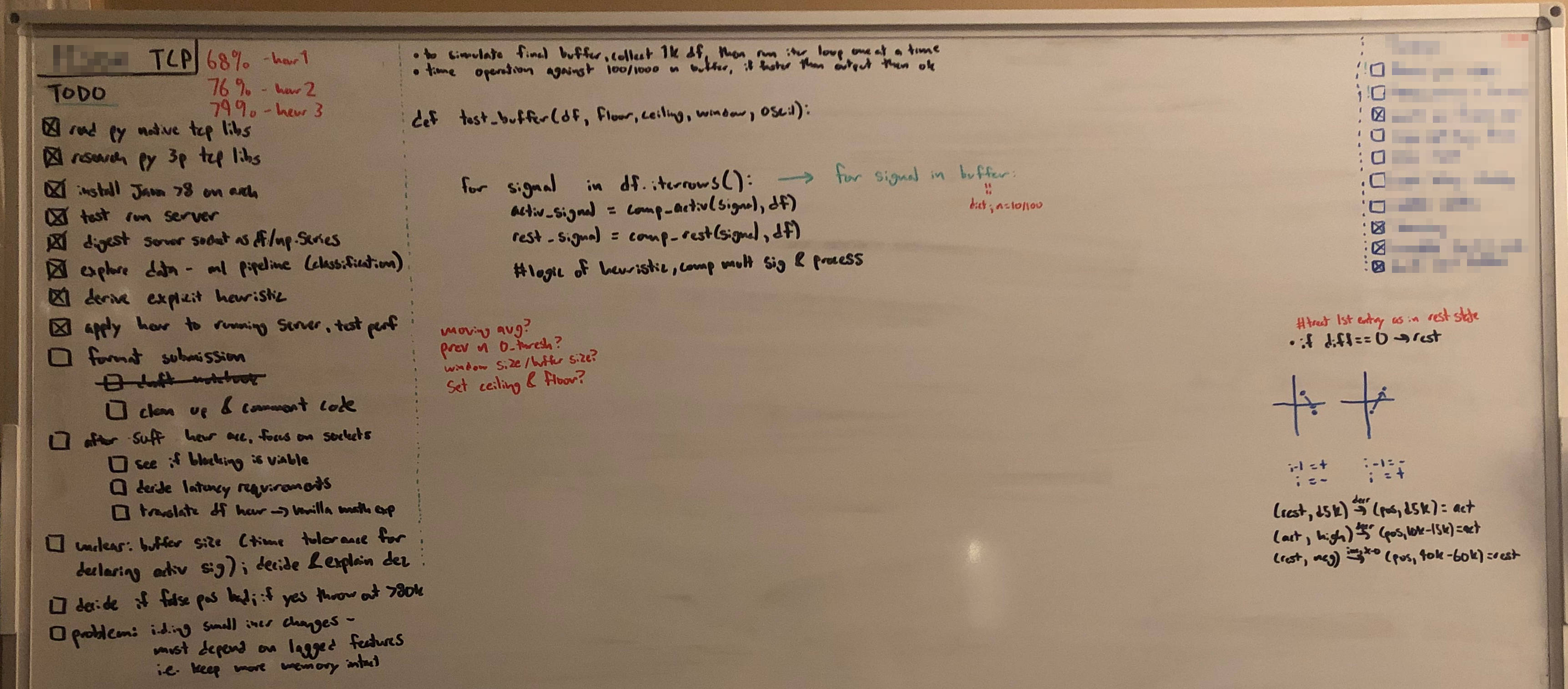
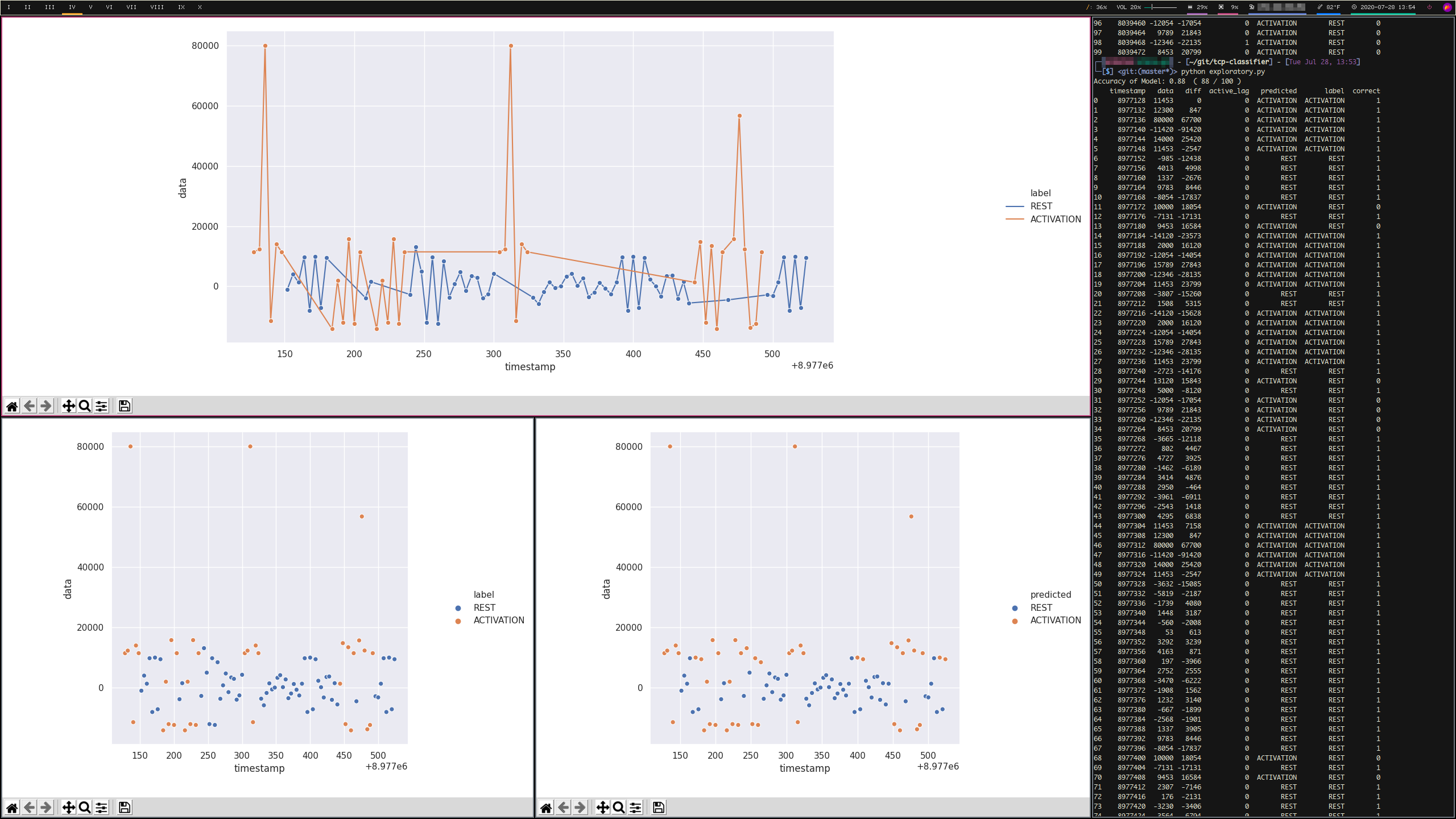
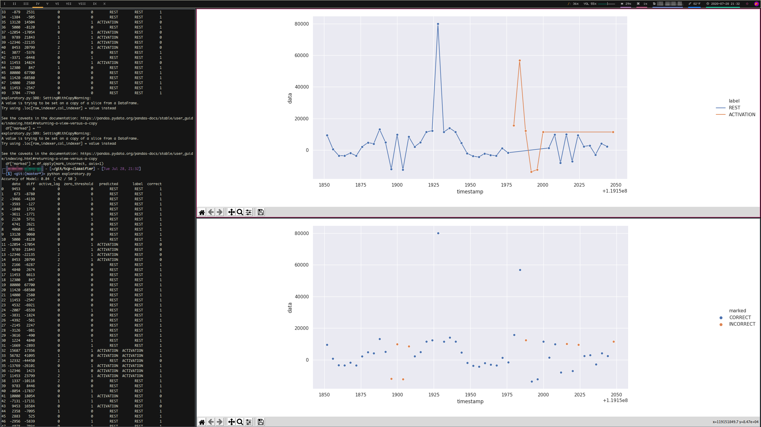
I purposefully left this file messy to make my process observable. It shows where I started with the problem. If you’d rather not install the graphing library seaborn, the below three images show my workflow for experimenting with labeling. In the first image, I kept track of ideas that I had for label rules while looking at the graphed true labels. In the second image, the generated graphs show the line plot of true signals above, and my predicted labels vs. true labels on scatter plots below. In the third image, I have a graph of the line plot of true signals above, and my correct vs. incorrect labels below.

intermediary.py

The purpose of this file is to test any heuristics developed in exploratory.py. There are two main distinguishing features compared to exploratory.py. First, I am timing the total elapsed time for each iteration. Second, I have set two parameters for the function that connects to the TCP socket. The parameter ‘n_iter’ is the length of the buffer which gets converted to a dataframe, and ‘n_epochs’ is the number of times the buffer will be generated. After the specified number of epochs have been run, the mean and median accuracy from every buffer is computed and output to the terminal. This allowed me to experiment with the how the size of buffer affected accuracy, as well as the actual accuracy of a given heuristic when run many more times than in exploratory.py.

tcp_classifier.py

This is the actual code submission, taking heuristic rules derived during exploration and applying them to the real-time data. The code has been commented and shortened for readability.

main.py

This is the file that executes tcp_classifier.py. If in future iterations there were multiple Python files that needed to interact with each other, they would be imported here. You could also run the program from the tcp_classifier.py file itself, centralizing project execution here reduces complexity if I continue to work on the project.

Design Considerations

Simple Heuristic vs. ML Classifier

Taking the recommendation from the challenge prompt, I opted to write my own set of rules to evaluate the data based on visualizations in the interest of time.

Performance - Accuracy & Speed

There were three iterations of heuristics completed for the project before a final ruleset was decided on, located in exploratory.py. Their accuracy was as follows:

• Heuristic 1: 68%
• Heuristic 2: 76%
• Heuristic 3: 79%
• Final Heuristic: 80%

These scores were calculated with intermediary.py, checked with the following parameter configurations:

• n_epochs=100 & n_iters=100
• n_epochs=100 & n_iters=1000
• n_epochs=1000 & n_iters=10

One interesting observation is that while the first three heuristics scored consistently at any of the above specified parameter values (for both mean and median accuracy), the final heuristic median accuracy varied noticeably with lower n_iters, hovering between 76%-90%.

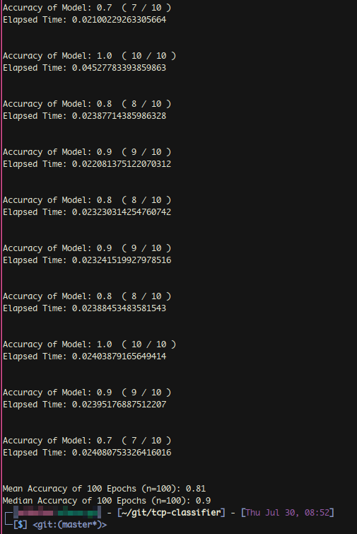
Measuring program speed in intermediary.py, total elapsed time from buffer ingestion to label output averaged 0.24 seconds with a buffer size of 100 data points, and 0.024 seconds with a buffer size of 10 data points (the final buffer sized used). The following screenshot shows intermediary.py in action.

Buffer & Epoch Size

While the epoch size did not affect measured performance after a sufficient value (~100), buffer size certainly did. This demonstrates the heuristic’s sensitivity to memory in the time series. While a buffer size of 100 pinned mean and median accuracy around 79%, reducing the buffer size to 10 increased mean accuracy but destabilized median results, as mentioned in the above section. The takeaway from this is that the extra memory with larger buffer sizes was not necessary to label the data, but additional rules would have to be added to the heuristic to reduce deviation in accuracy over the long-run. One other aspect not mentioned in the prompt but with real-world importance are latency requirements. Increased execution time by a factor of 10 linearly due to buffer size is probably not acceptable when digesting real-time data in production, so I decided to keep a lower buffer size for realism and accept the trade-off in variance.

Handling Exceptions

There are only two exceptions handled in tcp_classifier.py. A ‘JSONDecodeError’ in connect_socket() will simply discard the data, and a ‘KeyError’ in format_df() will similarly ignore that row when generating predicted labels.

False Positives

One flaw that becomes clear after looking at several graphs of the current predictions is that the ruleset does not reliably label data points in the 15,000 - 20,000 ‘data’ range, especially when a small incremental positive difference is followed by a large spike. The vast majority of the ~20% incorrect predictions occur here. Because I factor in the lagged activation in the rule set, any singular mis-labeled data before a large spike essentially guarantees a series of two to five incorrect predictions. I suspect additional rules factoring in features for crossing the x-axis, lagged small oscillations, or moving averages may alleviate this problem.

Moving Forward

If I were to work on this project for longer, I have a few additional ideas to explore. I would add additional scores to be returned by the function measure_performance() besides accuracy. For example, I could measure the differences in performance based on the window size of the buffer, a matrix of the rules triggered for each data point to minimize overlap, and the cost in time for each function as it is changed. The most important feature I would add to the function would be a confusion matrix to evaluate how false positives and negatives change with difference heuristics.

To achieve higher performance, I would experiment with machine learning classifiers. The PyTorch framework provides enough out-of-the-box support for common models that with another day or two I could most likely train a model with comparable or higher performance. Analyzing the rest/activation signals from graphed data by eyeballing it was quick and relatively effective, but after a couple hours there were no other rules for me to easily write based on graph interpretation. In this stage I would also generate more feature columns, such as the unused ‘zero_threshold’.

With more time, I would also change some of the design decisions that I made. For example, instead of discarding malformed data from the server (multiple non-separated messages), I would catch those exceptions with a separate function to unload into multiple JSON objects.

Final Submission

import json
import socket
import pandas as pd


# Prints a pandas dataframe in its entirely, instead of truncating rows with ellipses
def full_print_df(df):
    with pd.option_context('display.max_rows', None, 'display.max_columns', None):
        print(df)


# Converts a standard dictionary to a pandas dataframe
def format_df(raw_dict):
    df = pd.DataFrame.from_dict(raw_dict, orient='index')
    # Some dictionary elements are mis-formatted because of improperly received messages (zero or multiple data points)
    # This handles such exceptions and lets the malformed tuple through (it becomes discarded during analysis)
    try:
        df = df[df['timestamp'] != 0]
    except KeyError as e:
        cols = ['timestamp', 'data', 'label', 'predicted']
        df = pd.DataFrame(columns=cols)
        return df
    # Fills the column of predictions with rest state default
    df['predicted'] = "REST"

    return df


# Compute the lagged activation status for previous row(s), and fill the value for the current row
def apply_active_lag(df):
    for i in range(1, len(df)):
        if i == 0 or i == 1:
            df.loc[i, 'active_lag'] = 0
        elif df.loc[i - 1, 'predicted'] == "REST":
            df.loc[i, 'active_lag'] = 0
        elif df.loc[i - 1, 'predicted'] == "ACTIVATION" and df.loc[i - 2, 'predicted'] == "ACTIVATION":
            df.loc[i, 'active_lag'] = 2
        else:
            df.loc[i, 'active_lag'] = 1
    return df


# Compute the arithmetic difference of the current row from the previous row
def apply_diff_calc(df):
    for i in range(1, len(df)):
        df.loc[i, 'diff'] = df.loc[i, 'data'] - df.loc[i - 1, 'data']
    return df


# Compute if the current data value crossed 0 from the last data value, and fill the values
# This metric is not used in the current heuristic, but could potentially be useful
def apply_zero_threshold(df):
    for i in range(1, len(df)):
        if df.loc[i, 'data'] < 0 < df.loc[i - 1, 'data']:
            df.loc[i, 'zero_threshold'] = 1
        elif df.loc[i, 'data'] > 0 > df.loc[i - 1, 'data']:
            df.loc[i, 'zero_threshold'] = 1
        else:
            df.loc[i, 'zero_threshold'] = 0
    return df


# Apply the heuristic rules for making a prediction of a rest or activation state
# This is the final function that gets applied to the buffer
def apply_heuristic(row):
    # Large spikes not preceded by activation are predicted as rest
    if row['data'] >= 80000 and row['active_lag'] == 0:
        return "REST"
    # Initial entry is predicted as rest
    # (Not always true, but we weight lagged activation and can't afford to start the series with a false positive)
    elif row['diff'] == 0:
        return "REST"
    # Medium positive change in direction with positive data is activation
    elif row['diff'] > 10000 and row['data'] > 0:
        return "ACTIVATION"
    # Medium negative change in direction and previous activation is activation
    elif row['diff'] > -5000 and row['active_lag'] > 0:
        return "ACTIVATION"
    # Medium positive data or medium negative data is activation
    # This rule is problematic and requires more conditions to reduce false positives
    elif row['data'] > 15000 or row['data'] < -10000:
        return "ACTIVATION"
    # If no other rules are triggered, data is predicted as rest
    else:
        return "REST"


def heuristic(df):
    # Initializes new columns:
    # 1. The numerical difference data(n) - data(n-1)
    # 2. A lagged categorical variable for activation (values 0-2), to retain some memory of earlier predicted state
    # 3. A boolean variable for whether or not a data point crossed the x-axis from the n-1th data point
    df['diff'], df['active_lag'], df['zero_threshold'] = 0, 0, 0

    # Apply three functions that compute the above-initialized columns that will be used in the final apply_heuristic()
    df = apply_diff_calc(df=df)
    df = apply_active_lag(df=df)
    df = apply_zero_threshold(df=df)

    # Predict activation status based on the columns data, diff, and active_lag
    df['predicted'] = df.apply(apply_heuristic, axis=1)
    df = apply_active_lag(df=df)
    return df


# Returns a message to the TCP server if the predicted label is activated
def output_signal(df, socket_client):
    for index, row in df.iterrows():
        if row['predicted'] == 'ACTIVATION':
            socket_client.sendall(b'Activation classified\n')


# Input is a dictionary generated from the raw JSON data and the socket connection
# Populates a dataframe, applies the heuristic rule set, and calls the function to send a message for each activation
def read_buffer(buffer_dict, socket_client):
    df = format_df(raw_dict=buffer_dict)
    df = heuristic(df=df)
    output_signal(df=df, socket_client=socket_client)


# Opens the connection to the TCP server, and continuously ingests data in small buffers to analyze and label
def connect_socket():

    # Continuous loop that will not be broken unless the server closes the connect or a keyboard interruption is sent
    while True:
        # Initialize a counter and empty dictionary that get reset for each buffer
        i = 0
        d = {}

        # Initialize a socket connection on the specified port 7890
        s = socket.socket(socket.AF_INET, socket.SOCK_STREAM)
        s.connect(('localhost', 7890))

        # Inner continuous loop to generate a buffer where n=10
        while True:
            # Store the message received from the server, with a maximum size of 1024 bytes
            data = s.recv(1024)
            # When the counter reaches the buffer size (10), exit the inner continuous loop
            if i == 10:
                break
            # If the TCP server stops sending populated messages, exit the inner continuous loop
            if not data:
                break
            # Naively handling any messages that did not separate newlines
            # This is based on the assumption that false positives are less preferable than false negatives
            # With more time, a separate function to parse malformed messages could be executed instead of breaking
            try:
                formatted_data = json.loads(data)
            except json.decoder.JSONDecodeError as e:
                break

            # Populate the dictionary at index=i with the JSON-formatted data point {data:[], label:[], timestamp:[]}
            d[i] = formatted_data
            i += 1

        # Calls the function that handles formatting the dictionary, predicting labels, and sending back messages
        read_buffer(buffer_dict=d, socket_client=s)